
Self-Supervised Blind Denoising
12 June 2021
This post describes a novel state-of-the-art blind denoising method based on self-supervised deep neural networks[1] I am currently developing with Charles Ollion, Sylvain Le Corff (CMAP, Ecole Polytechnique, Université Paris-Saclay), Elisabeth Gassiat (Université Paris-Saclay, CNRS, Laboratoire de mathématiques d’Orsay) and Luc Lehéricy (Laboratoire J. A. Dieudonné, Université Côte d’Azur, CNRS). The preprint is available here: https://arxiv.org/abs/2102.08023

|
|
Introduction
- Our method is self-supervised, meaning that only a dataset of noisy images is sufficient to train the neural network (provided they are corrupted by the same process). This makes this method very useful when no pairs of high quality (clean) images + noisy images is available to train supervised methods such as CARE[3], which corresponds to most real-world use cases.
- Our method performs blind denoising: it doesn’t require a prior knowledge on the corruption process and is even able to characterize it.
- It is inspired by the recent Noise2Self[4] and Noise2Void[5] methods, and perform much better on all tested public datasets. It even performs better than the supervised method CARE[3].
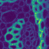
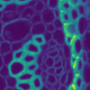
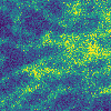
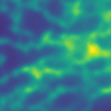
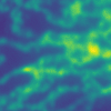
A good denoising method is able to efficiently reduce noise, without removing other high-frequency features such as gradients. As a comparison, Gaussian blur is one of the most simple and effective denoising method, but strongly affects gradients (i.e. the image looks blurred). The following figure displays the result of a Gaussian blur filter on the same image, with a scale adjusted so that the denoising efficiency is equivalent to our method. One can see how contrasts are much more reduced by Gaussian blur than by our method.
|
|

|
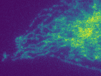
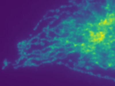
The figure below shows the result of our method on another dataset.
|

|
|
|
Details on the Method
The self-supervised training is inspired on the strategy developed in Noise2Self[4] and Noise2Void[5]; however those methods use a L2 objective function which intrinsically supposes that the noise process follows a Gaussian distribution. The novelty of our method is to add an auxiliary network (N-net) that recovers the noise distribution and enables to use a loss function corresponding to the actual noise distribution. We actually have shown that N-net accelerates and stabilizes the training of D-net. The denoising network (D-net) and N-net are trained simultaneously which makes this method very easy to train. This is a brief summary of our method, for more details see the preprint.
Notations:
- For all pixel locations
s in the image we have Ys = Xs + Ɛs - X
s denotes the signal value at locations - Y
s its noisy observation - Ɛ
s is the noise
Training setup
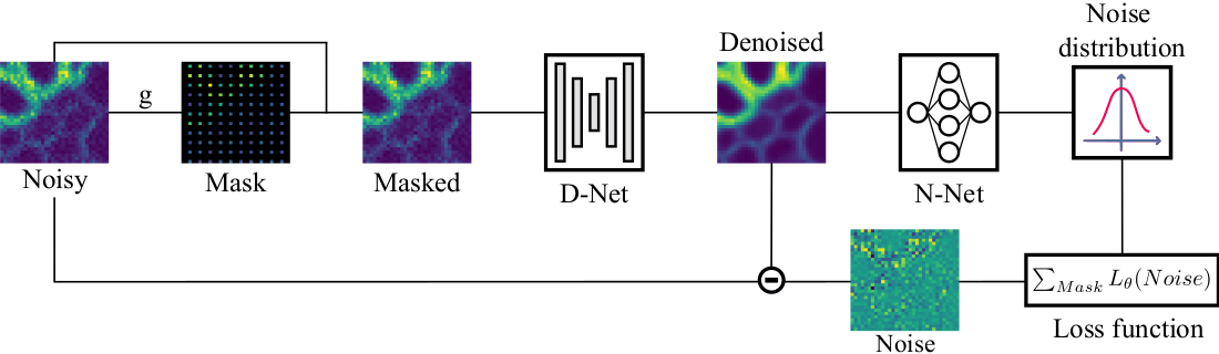
For each mini-batch, a random grid is drawn. The masking function is applied on each element of the grid, replacing the original pixels in the masked image by the average of its direct neighbors. The denoised image predicted by the D-net is fed to the N-net that predicts a noise distribution for each pixel. The loss function is then computed on each element of the grid.
Synthetic Noise Estimation
Clean images were corrupted with known noise distributions in order to evaluate the capacity of the N-net to recover noise distribution.
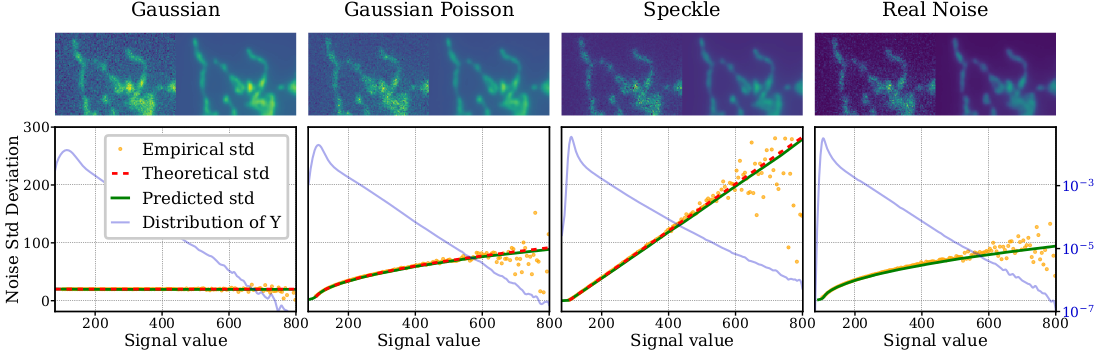
For 3 models of synthetic noise as well as the real noise, the plots display the empirical standard deviation of the noise Y - X, as well as the predicted standard deviation of the noise by the N-net as a function of X.
One of the most striking result of this experiment is that for the 3 cases of synthetic noise, the predicted standard deviation provided by the N-net is a very sharp approximation of the known theoretical standard deviation. It shows in particular that our method is able to capture the different noise distributions even in areas where signal is rare.
Improving Real Noise Estimation
We observed that contrary to the classical noise models considered in the denoising literature, real noise often displays a certain amount of skewness, as illustrated in the figure below. In order to be able to capture this aspect, we predict a Gaussian mixture model (GMM) instead of a simple Gaussian model.
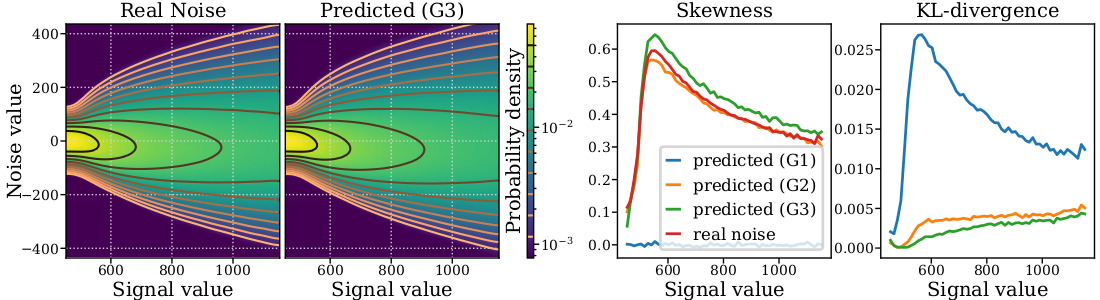
This Figure shows that noise skewness is well described by the predicted model, and the noise distribution is better described by a GMM than by a single Gaussian. This applies for all the considered datasets. In this example, it is interesting to note that the Kullback–Leibler divergence between the empirical noise distribution and the predicted distribution (as a function of the signal value) is improved by considering a GMM instead of a unimodal distribution. This supports the use of our flexible N-net to capture a large variety of noise distributions (with multimodality and/or skewness) which can be observed in experimental datasets.
Denoising performances and comparison with other methods
We compared our method to several baselines: D-net trained in a supervised setup with L2 objective (with all other training and prediction hyperparameters unchanged), N2V, DecoNoising[7], which is the self-supervised blind denoising method that has shown best results on the datasets we considered, as well as one of the most simple denoising method: convolution by a Gaussian, whose standard deviation is chosen to maximize the PSNR on the evaluation dataset. We believe the latter makes a good reference, as it is one of the simplest denoising methods, and it removes noise efficiently but also other high-frequency information such as local contrasts.
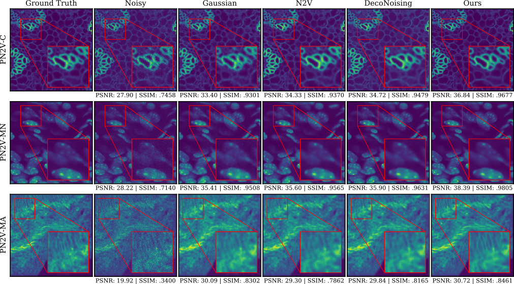
For the version predicting a simple Gaussian distribution, the average PSNR gain over DecoNoisng is +1.42dB. This is also confirmed by the visual aspect, displayed in the Figure above: our method produces images closer to the ground truth, smoother, sharper, more detailed and without visual artifacts. Remarkably, our method performs significantly better than the supervised method CARE[3], with an average PSNR gain of +1.49dB. Moreover, our method also performs better than its supervised counterpart with an average gain of +0.21dB. This could be explained by the fact that training with masking induces a lower dependency to central pixel compared to supervised training, and thus pushes the network to make better use of the neighborhood.
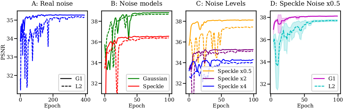
Impact of N-net on training
The N-net has a very significant impact on performances, in particular when training is short (e.g. as in N2V, N2S). We observe that the N-net greatly stabilizes the training and improves convergence speed (as illustrated in the figure below). As an illustration of the excellent training stability, we measured a SEM of 6x10⁻³ for the PSNR on dataset W2S-1 over 5 runs. We also observe that in all our hyperparameter settings that adding the N-net always improves performances over L2 objective, although not always significantly.
Conclusion
We introduced a novel self-supervised blind-denoising method modeling both the signal and the noise distributions. We believe its simplicity, performances and the interpretability of the noise distribution will be useful both in practical applications, and as a basis for future research.
References
-
J. Ollion, C. Ollion, E. Gassiat, L. Lehéricy, and S. L. Corff, “Joint self-supervised blind denoising and noise estimation,” arXiv preprint arXiv:2102.08023, 2021.
https://arxiv.org/abs/2102.08023 -
M. Prakash, M. Lalit, P. Tomancak, A. Krul, and F. Jug, “Fully unsupervised probabilistic noise2void,” in 2020 IEEE 17th International Symposium on Biomedical Imaging (ISBI), 2020, pp. 154–158.
-
M. Weigert et al., “Content-aware image restoration: pushing the limits of fluorescence microscopy,” Nature methods, vol. 15, no. 12, pp. 1090–1097, 2018.
-
J. Batson and L. Royer, “Noise2self: Blind denoising by self-supervision,” arXiv preprint arXiv:1901.11365, 2019.
https://arxiv.org/abs/1901.11365 -
A. Krull, T.-O. Buchholz, and F. Jug, “Noise2void-learning denoising from single noisy images,” in Proceedings of the IEEE Conference on Computer Vision and Pattern Recognition, 2019, pp. 2129–2137.
-
R. Zhou, M. E. Helou, D. Sage, T. Laroche, A. Seitz, and S. Süsstrunk, “W2S: A Joint Denoising and Super-Resolution Dataset,” arXiv preprint arXiv:2003.05961, 2020.
https://arxiv.org/abs/2003.05961 -
A. S. Goncharova, A. Honigmann, F. Jug, and A. Krull, “Improving Blind Spot Denoising for Microscopy,” 2020.